Gradient Descent Algorithm Explained

Often time, we need to find the minimum of a function, for example, in machine learning, we often need to minimize the loss function to improve the performance of our model. Gradient Descent is specifically designed to solve such optimization problems. Fundamentally, gradient descent seeks to find local minima of differntiable function, $f(x)$ by iteratively moving in the direction of the steepest descent as defined by the negative of the gradient.

Mathematics Technical Parts

Consider a differentiable function $f: \mathbb{R}^n \to \mathbb{R}$. The gradient of $f$ at a point $x \in \mathbb{R}^n$ is denoted as $\nabla f(x)$, which is a vector of partial derivatives. The gradient points in the direction of the steepest ascent of the function. To find a local minimum, we need to move in the opposite direction of the gradient. Hence, the exploits this by moving in the opposite direction:

$$x_{k+1} = x_k - \alpha \nabla f(x_k),$$

where:

• $x_k$ is the current point,
• $\alpha$ is the learning rate, where $\alpha > 0$,
• $\nabla f(x_k)$ is the gradient of $f$ at point $x_k$.

We simulate two different scenarios, one with postive gradient in loss function, and another with negative gradient in loss function.

Scenario 1: Positive Gradient

Let's consider a simple quadratic function:

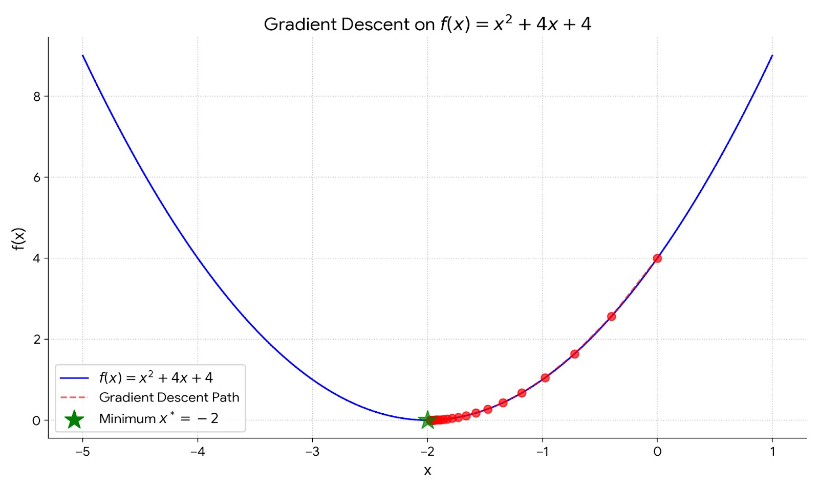
$$f(x) = x^2 + 4x + 4.$$

The gradient of this function is:

$$\nabla f(x) = 2x + 4.$$

Starting from an initial point, say $x_0 = 0$, and choosing a learning rate $\alpha = 0.1$, we can apply the gradient descent update rule iteratively:

1. Compute the gradient at the current point: $\nabla f(x_0) = 2(0) + 4 = 4$.
2. Update the point: $x_1 = x_0 - 0.1 \cdot 4 = 0 - 0.4 = -0.4$.
3. Repeat the process for a number of iterations.

For the first 5 iteration, we can tabulate the results as follows:

We can observe that the gradient os loss function from positive value is moving backward each time step, and the first step size is larger but it gradually decreases as we approach the minimum point. This is the brilliant part of gradient descent, as it automatically take larger steps when we are far from the minimum and smaller steps as we get closer to the minimum.

We can visualize the process using a simple plot:

import numpy as np
import matplotlib.pyplot as plt

# Define the function and its gradient
def f(x):
    return x**2 + 4*x + 4
def grad_f(x):
    return 2*x + 4

# Gradient Descent parameters
alpha = 0.1
x0 = 0
iterations = 20

# Store the points
x_points = [x0]
for _ in range(iterations):
    grad = grad_f(x_points[-1])
    x_new = x_points[-1] - alpha * grad
    x_points.append(x_new)

# Plotting
x = np.linspace(-5, 1, 100)
y = f(x)
plt.plot(x, y, label='f(x) = x^2 + 4x + 4')
plt.scatter(x_points, f(np.array(x_points)), color='red')
plt.plot(x_points, f(np.array(x_points)), color='red', linestyle='--', label='Gradient Descent Path')
plt.title('Gradient Descent on f(x)')
plt.xlabel('x')
plt.ylabel('f(x)')
plt.legend()
plt.grid()
plt.show()

After 20 iterations, the points converge towards the minimum point at $x = -2$. We can see how the points move along the curve of the function, gradually approaching the minimum.

Scenario 2: Negative Gradient

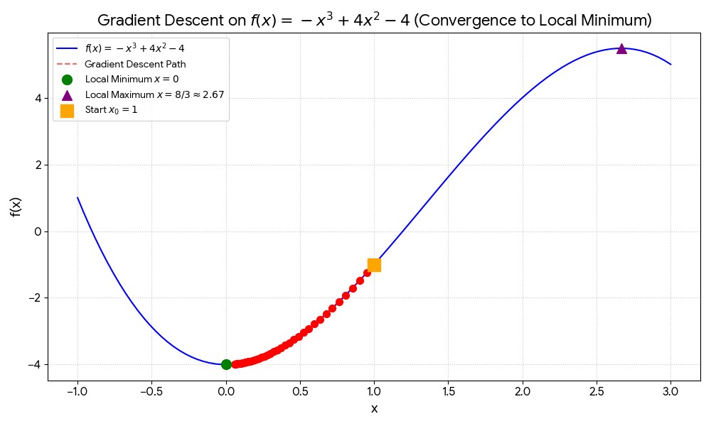
Now, let's consider a function with a negative gradient: $$f(x) = -x^3 + 4x^2 - 4.$$

The gradient of this function is: $$\nabla f(x) = -3x^2 + 8x.$$

Similar to what we have done on the previous example, we start from an initial point, say $x_0 = 0$, and choosing a learning rate $\alpha = 0.01$, we can apply the gradient descent update rule iteratively:

1. Compute the gradient at the current point: $\nabla f(x_0) = -3(0)^2 + 8(0) = 0$.
2. Update the point: $x_1 = x_0 - 0.01 \cdot 0 = 0$.
3. Repeat the process for a number of iterations.

For the first 5 iterations, we can tabulate the results as follows:

In this scenario, we can observe that the gradient of loss function from negative value is moving forward each time step, and the first step size is larger but it gradually decreases as we approach the minimum point. Similar to the previous scenario, gradient descent automatically adjusts the step size based on the distance from the minimum. Similarly, we can visualize the process using a simple plot:

import numpy as np
import matplotlib.pyplot as plt

# Define the function and its gradient
def f(x):
    return -x**3 + 4*x**2 - 4
def grad_f(x):
    return -3*x**2 + 8*x

# Gradient Descent parameters
alpha = 0.01
x0 = 1
iterations = 40

# Store the points
x_points = [x0]
for _ in range(iterations):
    grad = grad_f(x_points[-1])
    x_new = x_points[-1] - alpha * grad
    x_points.append(x_new)

# Plotting
x = np.linspace(-1, 3, 100)
y = f(x)
plt.plot(x, y, label='f(x) = -x^3 + 4x^2 - 4')
plt.scatter(x_points, f(np.array(x_points)), color='red')
plt.plot(x_points, f(np.array(x_points)), color='red', linestyle='--', label='Gradient Descent Path')
plt.title('Gradient Descent on f(x)')
plt.xlabel('x')
plt.ylabel('f(x)')
plt.legend()
plt.grid()
plt.show()

After 20 iterations, the points converge towards the minimum point at approximately $x = 0$. We can see how the points move along the curve of the function, gradually approaching the minimum. We plotted the gradient descent path on the function curve:

Proof of Convergence

To prove the convergence of the gradient descent algorithm, we need to show that the sequence of points generated by the algorithm converges to a local minimum of the function $f(x)$. We assume that $f$ is a convex function with Lipschitz continuous gradients, meaning there exists a constant $L > 0$ such that for all $x, y \in \mathbb{R}^n$, $$|\nabla f(x) - \nabla f(y)| \leq L |x - y|.$$

Under convexity alone, we show that the rate of convergence is sublinear. Specifically, we can show that after $k$ iterations, the function value satisfies:

$$ f(x_k) - f(x^*) \leq \frac{L |x_0-x^*|^2 }{2k}, $$

where $x^*$ is the global minimum point of $f$. This indicates that as the number of iterations $k$ increases, the function value approaches the minimum value at a rate inversely proportional to $k$.

This completes the proof of convergence for the gradient descent algorithm under the assumptions of convexity and Lipschitz continuous gradients. The algorithm effectively finds a local minimum of the function $f(x)$ by iteratively updating the points in the direction of the steepest descent.

But this is completely tied to the choice of learning rate $\alpha$. If $\alpha$ is too large, the algorithm may overshoot the minimum and diverge. If $\alpha$ is too small, the convergence will be very slow. Therefore, choosing an appropriate learning rate is crucial for the success of the gradient descent algorithm. They are various techniques to adaptively adjust the learning rate during the optimization process, such as learning rate schedules and adaptive optimization algorithms like Adam and RMSprop, which we can explore in future posts.

Known Issues of Gradient Descent

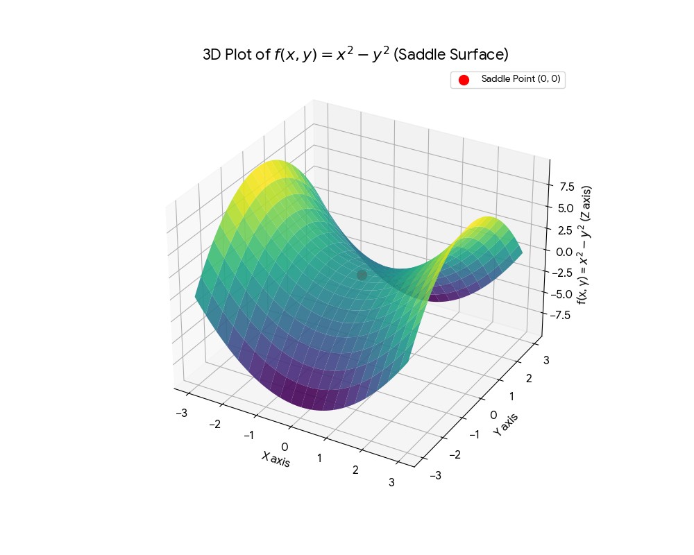
While gradient descent is a powerful optimization algorithm, it does have some known issues. In multivariate functions, the presence of saddle points can affect the convergence. Saddle points are points where the gradient is zero, but they are neither local minima nor local maxima. In high-dimensional spaces, saddle points are more prevalent than local minima, and gradient descent can get stuck at these points, leading to slow convergence or failure to find the global minimum. A popular example is the function $f(x, y) = x^2 - y^2$, which has a saddle point at $(0, 0)$. The direction vector at this point is zero, and gradient descent may struggle to escape this point.

To mitigate the issues with saddle points, various techniques can be employed, such as adding noise to the gradients, using momentum-based methods, or employing second-order optimization methods that consider the curvature of the function, which we can explore in future discussions. But overall, gradient descent remains a fundamental and widely used optimization algorithm in machine learning and various other fields.

Conclusion

Despite its simplicity, gradient descent is a powerful optimization algorithm that forms the backbone of many machine learning algorithms. By iteratively updating the parameters in the direction of the steepest descent, gradient descent effectively finds local minima of differentiable functions. Understanding its mathematical foundations and practical implementations is crucial for anyone working in the field of machine learning and optimization.

It's remarkable how such a simple iterative process can lead optimize almost any complex function in real life applications. I truly cannot appreciate enough the beauty of this elegant mathematical concept.

For those who are interested to learn more about gradient descent, I highly recommend watching the following video by StatQuest, which provides an excellent visual explanation of the algorithm:

I hope this post has provided a clear understanding of the gradient descent.